4.4. 演習:血液細胞計数#
顕微鏡画像の解析に深層学習を活用することで、作業の効率化が期待されています。例えば、基礎研究において、顕微鏡を使って細胞を種類ごとに分類し、その数を調べる作業が行われています。本節では、このような物体検出と個数カウントの実例として、顕微鏡で撮影した血液細胞の画像から赤血球、白血球、血小板を検出し、それぞれの個数を数える方法を学びます。
4.4.1. 演習準備#
4.4.1.1. ライブラリ#
本節で利用するライブラリを読み込みます。NumPy、Pnadas、Matplotlib、Pillow(PIL)などのライブライは、モデルの性能や推論結果などの可視化に利用します。scikit-learn(sklearn)、PyTorch(torch)、torchvision、torchmetrics は機械学習関連のライブラリであり、モデルの構築、検証や推論などに利用します。
import numpy as np
import pandas as pd
import matplotlib.pyplot as plt
import PIL.Image

import torch
import torchvision
import torchmetrics

print(f'torch v{torch.__version__}; torchvision v{torchvision.__version__}')
torch v2.8.0+cu126; torchvision v0.23.0+cu126
ライブラリの読み込み時に、ImportError や ModuleNotFoundError が発生した場合、必要なライブラリがインストールされていない可能性があります。該当ライブラリをインストールしてください。
4.4.1.2. データセット#
本節では、BCCD (blood cell count and detection) データセットを利用します。このデータセットは顕微鏡を利用して撮影された血液細胞の画像で、主に赤血球(red blood cell; RBC)、白血球(white blood cell; WBC)、血小板(platelet)を含みます。BCCD データセットは MIT ライセンスのもとで GitHub BCCD_Dataset で公開されており、著作権表示を行うことで自由に利用することができます。
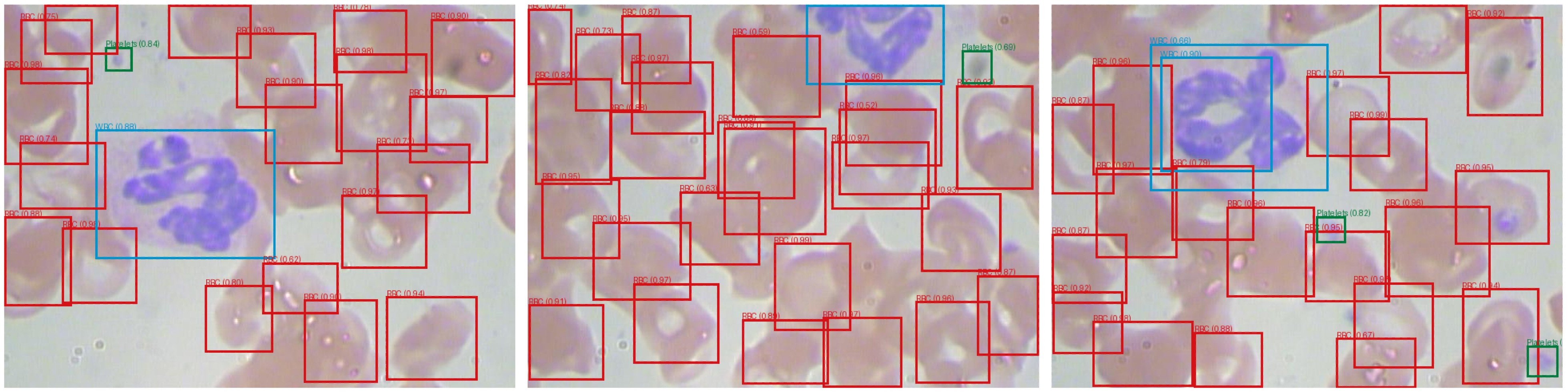
Fig. 4.12 BCCD データセットに含まれる顕微鏡画像のサンプル。#
本節では、オリジナルの BCCD データセットを再整理して作成したデータセットを利用します。本節で利用するデータセットは訓練、検証、そしてテストの 3 つのサブセットからなり、それぞれのサブセットにおいて各カテゴリに 50 枚、20 枚、20 枚の画像が含まれています。
Jupyter Notebook では、次のコマンドを実行することで、データをダウンロードできます。
!wget https://medDL.biopapyrus.jp/datasets/bccd.zip
!unzip bccd.zip
4.4.1.3. 前処理#
物体検出の問題では、画像と一緒に、検出対象の物体を囲むバウンディングボックスの座標とラベルをモデルに与え、学習させる必要があります。バウンディングボックスの座標とラベルは、一般的に COCO フォーマット(.json)や Pascal VOC フォーマット(.xml)などで保存されます。しかし、これらのフォーマットのままでは PyTorch で直接扱えないため、PyTorch が利用できる形式に変換する必要があります。
class CocoDataset(torchvision.datasets.CocoDetection):
    def __init__(self, root, annFile):
        super(CocoDataset, self).__init__(root, annFile)

    def __getitem__(self, idx):
        img, target = super(CocoDataset, self).__getitem__(idx)

        boxes = []
        labels = []
        for obj in target:
            bbox = obj['bbox']
            bbox = [bbox[0], bbox[1], bbox[0] + bbox[2], bbox[1] + bbox[3]]
            boxes.append(bbox)
            labels.append(obj['category_id'])

        img = torchvision.transforms.functional.to_tensor(img)
        target = {
            'boxes': torch.as_tensor(boxes, dtype=torch.float32),
            'labels': torch.as_tensor(labels, dtype=torch.int64),
        }

        return img, target
なお、画像分類と同様に、畳み込みニューラルネットワークでは入力する画像のサイズを指定されたサイズに変更する必要があります。ただし、このサイズ変更は CocoDetection 内で行われるため、ここであらためて設定する必要はありません。
また、モデルを訓練する際には、画像の拡大縮小や平行移動、回転などのデータ拡張を行い、それに伴ってバウンディングボックスの座標も同じように再計算する必要があります。しかし、これらの処理を加えるとコードが複雑化し、全体の流れがわかりにくくなるため、本節ではデータ拡張の処理は省略しています。
4.4.1.4. 計算デバイス#
PyTorch が GPU を認識できる場合は GPU を利用し、認識できない場合は CPU を利用するように計算デバイスを設定します。
device = torch.device('cuda') if torch.cuda.is_available() else torch.device('cpu')
4.4.2. モデル構築#
SSD(Single Shot MultiBox Detector)は、高性能な物体検出アーキテクチャであり、torchvision.models モジュールを通じて利用できます。しかし、このアーキテクチャは COCO データセット向けに設計されており、車や人などの 90 種類の一般的なオブジェクトを検出するための構造になっています。そのため、そのままでは血液細胞(赤血球、白血球、血小板)の検出には対応していません。
血液細胞の検出を行うには、このアーキテクチャの分類部分の出力数を、検出対象となる 3 カテゴリ(赤血球、白血球、血小板)に対応させる必要があります。この修正はモデルを呼び出すたびに同じ作業を繰り返す必要があり、手間がかかります。そこで、指定したクラス数に応じてアーキテクチャを生成し、必要に応じて修正を加えられるよう、一連の処理を関数として定義します。
def ssd(num_classes, weights=None):
    model = torchvision.models.detection.ssd300_vgg16(weights='DEFAULT')

    in_channels = torchvision.models.detection._utils.retrieve_out_channels(model.backbone, (300, 300))
    num_anchors = model.anchor_generator.num_anchors_per_location()
    model.head.classification_head = torchvision.models.detection.ssd.SSDClassificationHead(
        in_channels=in_channels,
        num_anchors=num_anchors,
        num_classes=num_classes + 1,
    )
    model.transform.min_size = (300,)
    model.transform.max_size = 3000
    if weights is not None:
        model.load_state_dict(torch.load(weights))
    return model

model = ssd(num_classes=3)
model.to(device)
Show code cell output
SSD(
  (backbone): SSDFeatureExtractorVGG(
    (features): Sequential(
      (0): Conv2d(3, 64, kernel_size=(3, 3), stride=(1, 1), padding=(1, 1))
      (1): ReLU(inplace=True)
      (2): Conv2d(64, 64, kernel_size=(3, 3), stride=(1, 1), padding=(1, 1))
      (3): ReLU(inplace=True)
      (4): MaxPool2d(kernel_size=2, stride=2, padding=0, dilation=1, ceil_mode=False)
      (5): Conv2d(64, 128, kernel_size=(3, 3), stride=(1, 1), padding=(1, 1))
      (6): ReLU(inplace=True)
      (7): Conv2d(128, 128, kernel_size=(3, 3), stride=(1, 1), padding=(1, 1))
      (8): ReLU(inplace=True)
      (9): MaxPool2d(kernel_size=2, stride=2, padding=0, dilation=1, ceil_mode=False)
      (10): Conv2d(128, 256, kernel_size=(3, 3), stride=(1, 1), padding=(1, 1))
      (11): ReLU(inplace=True)
      (12): Conv2d(256, 256, kernel_size=(3, 3), stride=(1, 1), padding=(1, 1))
      (13): ReLU(inplace=True)
      (14): Conv2d(256, 256, kernel_size=(3, 3), stride=(1, 1), padding=(1, 1))
      (15): ReLU(inplace=True)
      (16): MaxPool2d(kernel_size=2, stride=2, padding=0, dilation=1, ceil_mode=True)
      (17): Conv2d(256, 512, kernel_size=(3, 3), stride=(1, 1), padding=(1, 1))
      (18): ReLU(inplace=True)
      (19): Conv2d(512, 512, kernel_size=(3, 3), stride=(1, 1), padding=(1, 1))
      (20): ReLU(inplace=True)
      (21): Conv2d(512, 512, kernel_size=(3, 3), stride=(1, 1), padding=(1, 1))
      (22): ReLU(inplace=True)
    )
    (extra): ModuleList(
      (0): Sequential(
        (0): MaxPool2d(kernel_size=2, stride=2, padding=0, dilation=1, ceil_mode=False)
        (1): Conv2d(512, 512, kernel_size=(3, 3), stride=(1, 1), padding=(1, 1))
        (2): ReLU(inplace=True)
        (3): Conv2d(512, 512, kernel_size=(3, 3), stride=(1, 1), padding=(1, 1))
        (4): ReLU(inplace=True)
        (5): Conv2d(512, 512, kernel_size=(3, 3), stride=(1, 1), padding=(1, 1))
        (6): ReLU(inplace=True)
        (7): Sequential(
          (0): MaxPool2d(kernel_size=3, stride=1, padding=1, dilation=1, ceil_mode=False)
          (1): Conv2d(512, 1024, kernel_size=(3, 3), stride=(1, 1), padding=(6, 6), dilation=(6, 6))
          (2): ReLU(inplace=True)
          (3): Conv2d(1024, 1024, kernel_size=(1, 1), stride=(1, 1))
          (4): ReLU(inplace=True)
        )
      )
      (1): Sequential(
        (0): Conv2d(1024, 256, kernel_size=(1, 1), stride=(1, 1))
        (1): ReLU(inplace=True)
        (2): Conv2d(256, 512, kernel_size=(3, 3), stride=(2, 2), padding=(1, 1))
        (3): ReLU(inplace=True)
      )
      (2): Sequential(
        (0): Conv2d(512, 128, kernel_size=(1, 1), stride=(1, 1))
        (1): ReLU(inplace=True)
        (2): Conv2d(128, 256, kernel_size=(3, 3), stride=(2, 2), padding=(1, 1))
        (3): ReLU(inplace=True)
      )
      (3-4): 2 x Sequential(
        (0): Conv2d(256, 128, kernel_size=(1, 1), stride=(1, 1))
        (1): ReLU(inplace=True)
        (2): Conv2d(128, 256, kernel_size=(3, 3), stride=(1, 1))
        (3): ReLU(inplace=True)
      )
    )
  )
  (anchor_generator): DefaultBoxGenerator(aspect_ratios=[[2], [2, 3], [2, 3], [2, 3], [2], [2]], clip=True, scales=[0.07, 0.15, 0.33, 0.51, 0.69, 0.87, 1.05], steps=[8, 16, 32, 64, 100, 300])
  (head): SSDHead(
    (classification_head): SSDClassificationHead(
      (module_list): ModuleList(
        (0): Conv2d(512, 16, kernel_size=(3, 3), stride=(1, 1), padding=(1, 1))
        (1): Conv2d(1024, 24, kernel_size=(3, 3), stride=(1, 1), padding=(1, 1))
        (2): Conv2d(512, 24, kernel_size=(3, 3), stride=(1, 1), padding=(1, 1))
        (3): Conv2d(256, 24, kernel_size=(3, 3), stride=(1, 1), padding=(1, 1))
        (4-5): 2 x Conv2d(256, 16, kernel_size=(3, 3), stride=(1, 1), padding=(1, 1))
      )
    )
    (regression_head): SSDRegressionHead(
      (module_list): ModuleList(
        (0): Conv2d(512, 16, kernel_size=(3, 3), stride=(1, 1), padding=(1, 1))
        (1): Conv2d(1024, 24, kernel_size=(3, 3), stride=(1, 1), padding=(1, 1))
        (2): Conv2d(512, 24, kernel_size=(3, 3), stride=(1, 1), padding=(1, 1))
        (3): Conv2d(256, 24, kernel_size=(3, 3), stride=(1, 1), padding=(1, 1))
        (4-5): 2 x Conv2d(256, 16, kernel_size=(3, 3), stride=(1, 1), padding=(1, 1))
      )
    )
  )
  (transform): GeneralizedRCNNTransform(
      Normalize(mean=[0.48235, 0.45882, 0.40784], std=[0.00392156862745098, 0.00392156862745098, 0.00392156862745098])
      Resize(min_size=(300,), max_size=3000, mode='bilinear')
  )
)
4.4.3. モデル訓練#
モデルが学習データを効率よく学習できるようにするため、学習アルゴリズム(optimizer)、学習率(lr)、および学習率を調整するスケジューラ(lr_scheduler)を設定します。
optimizer = torch.optim.AdamW(model.parameters(), lr=1e-4, weight_decay=1e-4)
lr_scheduler = torch.optim.lr_scheduler.StepLR(optimizer, step_size=3, gamma=0.1)
次に、訓練データと検証データを読み込み、モデルが入力できる形式に整えます。
train_loader = torch.utils.data.DataLoader(
                    CocoDataset('bccd', 'bccd/train.bbox.json'),
                    batch_size=4, shuffle=True, collate_fn=lambda x: tuple(zip(*x)))
valid_loader = torch.utils.data.DataLoader(
                    CocoDataset('bccd', 'bccd/valid.bbox.json'),
                    batch_size=4, shuffle=False, collate_fn=lambda x: tuple(zip(*x)))
Show code cell output
loading annotations into memory...
Done (t=0.00s)
creating index...
index created!
loading annotations into memory...
Done (t=0.00s)
creating index...
index created!
準備が整ったら、訓練を開始します。訓練プロセスでは、訓練と検証を交互に繰り返します。訓練では、訓練データを使ってモデルのパラメータを更新し、その際の損失(誤差)を記録します。検証では、検証データを使ってモデルの予測性能(mAP)を計算し、その結果を記録します。
num_epochs = 10
metric_dict = []

for epoch in range(num_epochs):
    # training phase
    model.train()
    epoch_loss_dict = {}

    for images, targets in train_loader:
        images = [img.to(device) for img in images]
        targets = [{k: v.to(device) for k, v in t.items()} for t in targets]

        batch_loss_dict = model(images, targets)
        batch_tol_loss = 0
        for loss_type, loss_val in batch_loss_dict.items():
            batch_tol_loss += loss_val
            if loss_type in epoch_loss_dict:
                epoch_loss_dict[f'train_{loss_type}'] += loss_val.item()
            else:
                epoch_loss_dict[f'train_{loss_type}'] = loss_val.item()

        # update weights
        optimizer.zero_grad()
        batch_tol_loss.backward()
        optimizer.step()
    lr_scheduler.step()

    # validation phase
    model.eval()
    metric = torchmetrics.detection.mean_ap.MeanAveragePrecision()
    with torch.no_grad():
        for images, targets in valid_loader:
            images = [img.to(device) for img in images]
            targets = [{k: v.to(device) for k, v in t.items()} for t in targets]
            metric.update(model(images), targets)


    # record training loss
    epoch_loss_dict['train_loss_total'] = sum(epoch_loss_dict.values())
    metric_dict.append({k: v / len(train_loader) for k, v in epoch_loss_dict.items()})
    for k, v in metric.compute().items():
        if k != 'classes':
            metric_dict[-1][k] = v.item()
    metric_dict[-1]['epoch'] = epoch + 1

    print(metric_dict[-1])
Show code cell output
{'train_bbox_regression': 0.07671675773767325, 'train_classification': 0.34619896228496844, 'train_loss_total': 0.4229157200226417, 'map': 0.07692664116621017, 'map_50': 0.17916372418403625, 'map_75': 0.05351657047867775, 'map_small': 0.00032615027157589793, 'map_medium': 0.07595260441303253, 'map_large': 0.1402052640914917, 'mar_1': 0.018004534766077995, 'mar_10': 0.12563492357730865, 'mar_100': 0.24816779792308807, 'mar_small': 0.07999999821186066, 'mar_medium': 0.20277777314186096, 'mar_large': 0.38410714268684387, 'map_per_class': -1.0, 'mar_100_per_class': -1.0, 'epoch': 1}
{'train_bbox_regression': 0.0623809053347661, 'train_classification': 0.28523656038137585, 'train_loss_total': 0.34761746571614194, 'map': 0.12759172916412354, 'map_50': 0.2719613015651703, 'map_75': 0.1029098629951477, 'map_small': 0.0002436571812722832, 'map_medium': 0.1482943445444107, 'map_large': 0.2121739536523819, 'mar_1': 0.026825396344065666, 'mar_10': 0.15972788631916046, 'mar_100': 0.26280951499938965, 'mar_small': 0.05999999865889549, 'mar_medium': 0.22936508059501648, 'mar_large': 0.4120238125324249, 'map_per_class': -1.0, 'mar_100_per_class': -1.0, 'epoch': 2}
{'train_bbox_regression': 0.04634404640931349, 'train_classification': 0.24762544265160194, 'train_loss_total': 0.2939694890609154, 'map': 0.235687255859375, 'map_50': 0.5231779217720032, 'map_75': 0.1363225132226944, 'map_small': 0.0, 'map_medium': 0.19141194224357605, 'map_large': 0.3716762065887451, 'mar_1': 0.12985260784626007, 'mar_10': 0.23783446848392487, 'mar_100': 0.3513605296611786, 'mar_small': 0.0, 'mar_medium': 0.2700396776199341, 'mar_large': 0.5316666960716248, 'map_per_class': -1.0, 'mar_100_per_class': -1.0, 'epoch': 3}
{'train_bbox_regression': 0.06048080554375282, 'train_classification': 0.23007093943082368, 'train_loss_total': 0.29055174497457653, 'map': 0.26107558608055115, 'map_50': 0.5059975981712341, 'map_75': 0.21528738737106323, 'map_small': 0.0, 'map_medium': 0.19805613160133362, 'map_large': 0.4091687500476837, 'mar_1': 0.15663264691829681, 'mar_10': 0.2732766568660736, 'mar_100': 0.36155328154563904, 'mar_small': 0.0, 'mar_medium': 0.25734126567840576, 'mar_large': 0.5548214316368103, 'map_per_class': -1.0, 'mar_100_per_class': -1.0, 'epoch': 4}
{'train_bbox_regression': 0.05030577457868136, 'train_classification': 0.2243338915017935, 'train_loss_total': 0.27463966608047485, 'map': 0.2791653871536255, 'map_50': 0.5236508250236511, 'map_75': 0.24081262946128845, 'map_small': 0.0, 'map_medium': 0.2004363238811493, 'map_large': 0.4382939338684082, 'mar_1': 0.16674603521823883, 'mar_10': 0.27605441212654114, 'mar_100': 0.36367347836494446, 'mar_small': 0.0, 'mar_medium': 0.2561507821083069, 'mar_large': 0.5594047904014587, 'map_per_class': -1.0, 'mar_100_per_class': -1.0, 'epoch': 5}
{'train_bbox_regression': 0.04262045713571402, 'train_classification': 0.22091278663048378, 'train_loss_total': 0.2635332437661978, 'map': 0.30708515644073486, 'map_50': 0.5335981845855713, 'map_75': 0.32128843665122986, 'map_small': 0.0, 'map_medium': 0.20060096681118011, 'map_large': 0.47948595881462097, 'mar_1': 0.1881859451532364, 'mar_10': 0.29908162355422974, 'mar_100': 0.3664059042930603, 'mar_small': 0.0, 'mar_medium': 0.2569444477558136, 'mar_large': 0.5603571534156799, 'map_per_class': -1.0, 'mar_100_per_class': -1.0, 'epoch': 6}
{'train_bbox_regression': 0.03483042350182167, 'train_classification': 0.21755363390995905, 'train_loss_total': 0.2523840574117807, 'map': 0.30817270278930664, 'map_50': 0.5346719622612, 'map_75': 0.320916086435318, 'map_small': 0.0, 'map_medium': 0.20074987411499023, 'map_large': 0.48154473304748535, 'mar_1': 0.1881859451532364, 'mar_10': 0.2991950213909149, 'mar_100': 0.3662925064563751, 'mar_small': 0.0, 'mar_medium': 0.2537698447704315, 'mar_large': 0.5624404549598694, 'map_per_class': -1.0, 'mar_100_per_class': -1.0, 'epoch': 7}
{'train_bbox_regression': 0.04371947508591872, 'train_classification': 0.22681008852445161, 'train_loss_total': 0.27052956361037034, 'map': 0.30889901518821716, 'map_50': 0.53492271900177, 'map_75': 0.32148998975753784, 'map_small': 0.0, 'map_medium': 0.20024940371513367, 'map_large': 0.48318731784820557, 'mar_1': 0.1881859451532364, 'mar_10': 0.2993083894252777, 'mar_100': 0.3664059042930603, 'mar_small': 0.0, 'mar_medium': 0.25337302684783936, 'mar_large': 0.5630357265472412, 'map_per_class': -1.0, 'mar_100_per_class': -1.0, 'epoch': 8}
{'train_bbox_regression': 0.037937939167022705, 'train_classification': 0.22206209256098822, 'train_loss_total': 0.2600000317280109, 'map': 0.30227333307266235, 'map_50': 0.533718466758728, 'map_75': 0.322264164686203, 'map_small': 0.0, 'map_medium': 0.2004343569278717, 'map_large': 0.4729100167751312, 'mar_1': 0.18307256698608398, 'mar_10': 0.2941950261592865, 'mar_100': 0.36727890372276306, 'mar_small': 0.0, 'mar_medium': 0.25257936120033264, 'mar_large': 0.564047634601593, 'map_per_class': -1.0, 'mar_100_per_class': -1.0, 'epoch': 9}
{'train_bbox_regression': 0.03832838856256925, 'train_classification': 0.22216596970191368, 'train_loss_total': 0.2604943582644829, 'map': 0.3025713562965393, 'map_50': 0.5337430834770203, 'map_75': 0.3224107325077057, 'map_small': 0.0, 'map_medium': 0.20048457384109497, 'map_large': 0.47364404797554016, 'mar_1': 0.18307256698608398, 'mar_10': 0.2944217622280121, 'mar_100': 0.36750566959381104, 'mar_small': 0.0, 'mar_medium': 0.25257936120033264, 'mar_large': 0.5646428465843201, 'map_per_class': -1.0, 'mar_100_per_class': -1.0, 'epoch': 10}
訓練後、訓練中の損失および検証性能の変化を可視化し、訓練が正しく行われたかどうかを確認します。
Show code cell source
metric_dict = pd.DataFrame(metric_dict)

fig, ax = plt.subplots(1, 2)
ax[0].plot(metric_dict['epoch'], metric_dict['train_loss_total'], label='total')
ax[0].plot(metric_dict['epoch'], metric_dict['train_classification'], label='classification')
ax[0].plot(metric_dict['epoch'], metric_dict['train_bbox_regression'], label='bbox')
ax[0].set_xlabel('epoch')
ax[0].set_ylabel('loss')
ax[0].set_title('Train')
ax[0].legend()
ax[1].plot(metric_dict['epoch'], metric_dict['map_50'])
ax[1].set_ylim(0, 1)
ax[1].set_xlabel('epoch')
ax[1].set_ylabel('mAP (50%)')
ax[1].set_title('Validation')
plt.tight_layout()
fig.show()
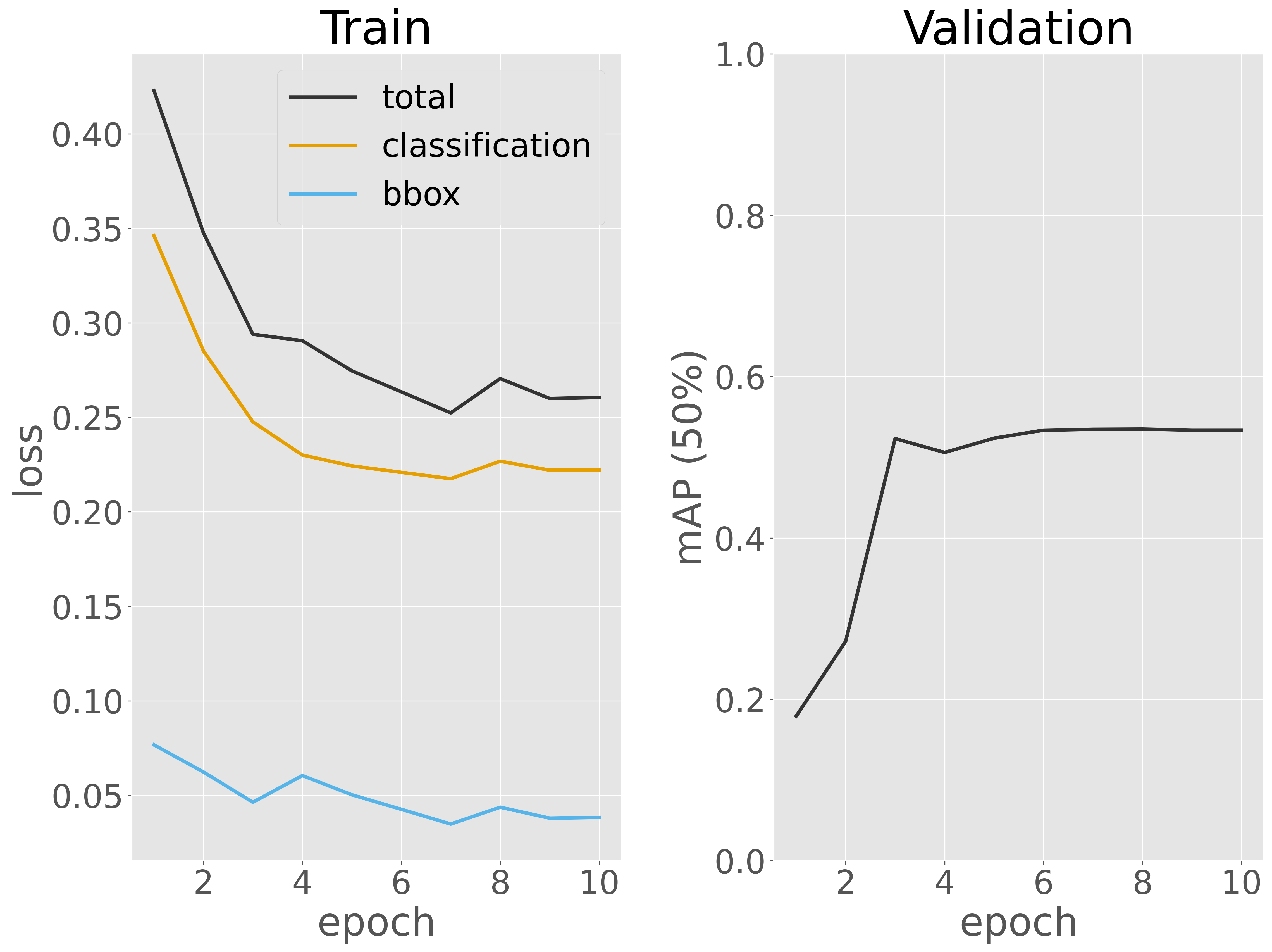
訓練データに対する損失はエポック数の増加に伴って徐々に減少しており、一部で上下するものの、後半では収束しているように見えます。また、検証データに対する検出性能(mAP 50%)は、4 エポック目以降安定して 前後で推移しています。この結果から、さらなる性能改善を目指す場合には、データセットを増やしたりする必要があるかもしれません。ただし、本節では時間の関係上、ここで訓練を終了します。
次に、この手順を Faster R-CNN や YOLO など、他の深層ニューラルネットワークアーキテクチャに適用し、それぞれの検証性能を比較して、このデータセットに最適なアーキテクチャを選定するプロセスを考えます。ただし、本節では時間の都合上、他のアーキテクチャを構築せず、既に構築した SSD を最適なアーキテクチャと仮定して次のステップに進みます。
次のステップでは、訓練サブセットと検証サブセットを統合したデータセット(trainvalid.bbox.json)を用いて、最適と判断したアーキテクチャを最初から訓練します。
# model
model = ssd(num_classes=3)
model.to(device)

# training parameters
optimizer = torch.optim.AdamW(model.parameters(), lr=1e-4, weight_decay=1e-4)
lr_scheduler = torch.optim.lr_scheduler.StepLR(optimizer, step_size=3, gamma=0.1)

# training data
train_loader = torch.utils.data.DataLoader(
                    CocoDataset('bccd', 'bccd/trainvalid.bbox.json'),
                    batch_size=4, shuffle=True, collate_fn=lambda x: tuple(zip(*x)))

# training
num_epochs = 5
metric_dict = []
for epoch in range(num_epochs):
    model.train()
    epoch_loss_dict = {}
    for images, targets in train_loader:
        images = [img.to(device) for img in images]
        targets = [{k: v.to(device) for k, v in t.items()} for t in targets]

        batch_loss_dict = model(images, targets)
        batch_tol_loss = 0
        for loss_type, loss_val in batch_loss_dict.items():
            batch_tol_loss += loss_val
            if loss_type in epoch_loss_dict:
                epoch_loss_dict[f'train_{loss_type}'] += loss_val.item()
            else:
                epoch_loss_dict[f'train_{loss_type}'] = loss_val.item()

        # update weights
        optimizer.zero_grad()
        batch_tol_loss.backward()
        optimizer.step()
    lr_scheduler.step()

    # record training loss
    epoch_loss_dict['train_loss_total'] = sum(epoch_loss_dict.values())
    metric_dict.append({k: v / len(train_loader) for k, v in epoch_loss_dict.items()})
    metric_dict[-1]['epoch'] = epoch + 1

    print(metric_dict[-1])
Show code cell output
loading annotations into memory...
Done (t=0.00s)
creating index...
index created!
{'train_bbox_regression': 0.05917167001300388, 'train_classification': 0.23940436045328775, 'train_loss_total': 0.29857603046629166, 'epoch': 1}
{'train_bbox_regression': 0.03635381990008884, 'train_classification': 0.20590729183620876, 'train_loss_total': 0.2422611117362976, 'epoch': 2}
{'train_bbox_regression': 0.036276178227530584, 'train_classification': 0.15656096405453152, 'train_loss_total': 0.1928371422820621, 'epoch': 3}
{'train_bbox_regression': 0.025822818279266357, 'train_classification': 0.14526267846425375, 'train_loss_total': 0.1710854967435201, 'epoch': 4}
{'train_bbox_regression': 0.030168516768349543, 'train_classification': 0.14405002858903673, 'train_loss_total': 0.17421854535738626, 'epoch': 5}
訓練が完了したら、訓練済みモデルの重みをファイルに保存します。
model.to('cpu')
torch.save(model.state_dict(), 'bccd.pth')
4.4.4. モデル評価#
最適なモデルが得られたら、次にテストデータを用いてモデルを詳細に評価します。
test_loader = torch.utils.data.DataLoader(
                    CocoDataset('bccd', 'bccd/test.bbox.json'),
                    batch_size=4, shuffle=False, collate_fn=lambda x: tuple(zip(*x)))

model = ssd(num_classes=3, weights='bccd.pth')
model.to(device)
model.eval()

n_cells = [[], [], []]
n_pred_cells = [[], [], []]

metric = torchmetrics.detection.mean_ap.MeanAveragePrecision()
with torch.no_grad():
    for images, targets in test_loader:
        images = [img.to(device) for img in images]
        targets = [{k: v.to(device) for k, v in t.items()} for t in targets]
        outputs = model(images)

        for target, output in zip(targets, outputs):
            n_cells_ = [0, 0, 0]
            n_pred_cells_ = [0, 0, 0]
            for label in target['labels']:
                n_cells_[label.item() - 1] += 1
            for label, score in zip(output['labels'], output['scores']):
                if score > 0.5:
                    n_pred_cells_[label.item() - 1] += 1
            for i in range(3):
                n_cells[i].append(n_cells_[i])
                n_pred_cells[i].append(n_pred_cells_[i])
        metric.update(outputs, targets)

n_cells = pd.DataFrame(n_cells, index=['WBC', 'RBC', 'Platelets']).T
n_pred_cells = pd.DataFrame(n_pred_cells, index=['WBC', 'RBC', 'Platelets']).T

metrics = {}
for k, v in metric.compute().items():
    metrics[k] = v.cpu().detach().numpy().tolist()
Show code cell output
loading annotations into memory...
Done (t=0.00s)
creating index...
index created!
metrics
{'map': 0.3847399652004242,
 'map_50': 0.6233562231063843,
 'map_75': 0.4637047350406647,
 'map_small': -1.0,
 'map_medium': 0.28021302819252014,
 'map_large': 0.5852371454238892,
 'mar_1': 0.23062728345394135,
 'mar_10': 0.4743475317955017,
 'mar_100': 0.6063894629478455,
 'mar_small': -1.0,
 'mar_medium': 0.5180583000183105,
 'mar_large': 0.6624394655227661,
 'map_per_class': -1.0,
 'mar_100_per_class': -1.0,
 'classes': [1, 2, 3]}
テストデータに対する検出性能を確認したところ、mAP(50%)が 0.623 程度であり、まだ改善の余地があるかもしれません。時間の関係上、モデルのチューニングをここで終了します。次に、モデルが予測した細胞の数と、実際にアノテーションされた細胞の数を比較するために、画像上で結果を可視化します。
fig, ax = plt.subplots()
for i in range(3):
    ax.scatter(n_cells.iloc[:, i], n_pred_cells.iloc[:, i], label=n_cells.columns[i], alpha=0.5)
ax.set_xlabel('Number of Cells')
ax.set_ylabel('Number of Predicted Cells')
ax.set_aspect('equal')
ax.legend()
fig.show()
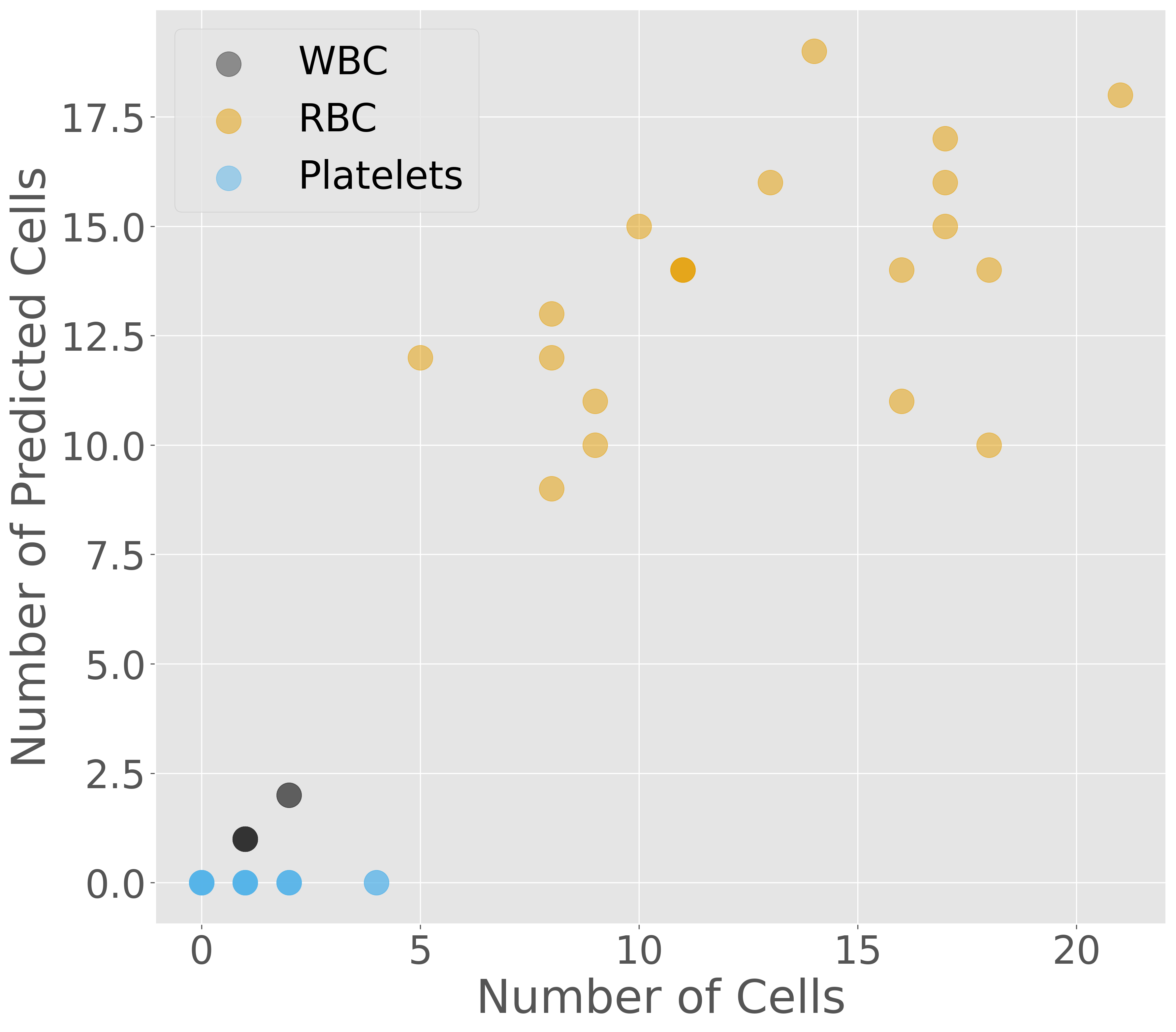
可視化の結果、白血球と赤血球の予測数はアノテーションされた数と似た数となることを確認できます。しかし、血小板についてはほとんど予測できていないことがわかります。これをより正確に評価するには、RMSE(平方平均二乗誤差)などの指標を用いる必要がありますが、ここで省略します。
血小板の予測が困難だった理由の一つは、SSD が持つ特徴と考えられます。SSD は大きな物体を高速かつ高精度で検出するのに優れている一方で、血小板のような小さな物体の検出は得意ではありません。また、今回使用したデータセットでは、血小板のアノテーション数が非常に少なかったことも影響していると考えられます。その結果、SSD は血小板のような小さな物体の特徴を十分に学習できなかった可能性があります。このように、大きな物体と小さな物体が混在する画像で、特に小さな物体のアノテーション数が著しく少ない場合、SSD は必ずしも最適な選択ではないと考えられます。
4.4.5. 推論#
推論時にも、訓練時と同じように torchvision モジュールからアーキテクチャを呼び出し、出力層のクラス数を設定します。その後、load_state_dict メソッドを使って、訓練済みの重みファイルをモデルにロードします。これらの操作はすべて ssd 関数で定義されているので、その関数を利用します。
model = ssd(num_classes=3, weights='bccd.pth')
model.to(device)
model.eval()
Show code cell output
SSD(
  (backbone): SSDFeatureExtractorVGG(
    (features): Sequential(
      (0): Conv2d(3, 64, kernel_size=(3, 3), stride=(1, 1), padding=(1, 1))
      (1): ReLU(inplace=True)
      (2): Conv2d(64, 64, kernel_size=(3, 3), stride=(1, 1), padding=(1, 1))
      (3): ReLU(inplace=True)
      (4): MaxPool2d(kernel_size=2, stride=2, padding=0, dilation=1, ceil_mode=False)
      (5): Conv2d(64, 128, kernel_size=(3, 3), stride=(1, 1), padding=(1, 1))
      (6): ReLU(inplace=True)
      (7): Conv2d(128, 128, kernel_size=(3, 3), stride=(1, 1), padding=(1, 1))
      (8): ReLU(inplace=True)
      (9): MaxPool2d(kernel_size=2, stride=2, padding=0, dilation=1, ceil_mode=False)
      (10): Conv2d(128, 256, kernel_size=(3, 3), stride=(1, 1), padding=(1, 1))
      (11): ReLU(inplace=True)
      (12): Conv2d(256, 256, kernel_size=(3, 3), stride=(1, 1), padding=(1, 1))
      (13): ReLU(inplace=True)
      (14): Conv2d(256, 256, kernel_size=(3, 3), stride=(1, 1), padding=(1, 1))
      (15): ReLU(inplace=True)
      (16): MaxPool2d(kernel_size=2, stride=2, padding=0, dilation=1, ceil_mode=True)
      (17): Conv2d(256, 512, kernel_size=(3, 3), stride=(1, 1), padding=(1, 1))
      (18): ReLU(inplace=True)
      (19): Conv2d(512, 512, kernel_size=(3, 3), stride=(1, 1), padding=(1, 1))
      (20): ReLU(inplace=True)
      (21): Conv2d(512, 512, kernel_size=(3, 3), stride=(1, 1), padding=(1, 1))
      (22): ReLU(inplace=True)
    )
    (extra): ModuleList(
      (0): Sequential(
        (0): MaxPool2d(kernel_size=2, stride=2, padding=0, dilation=1, ceil_mode=False)
        (1): Conv2d(512, 512, kernel_size=(3, 3), stride=(1, 1), padding=(1, 1))
        (2): ReLU(inplace=True)
        (3): Conv2d(512, 512, kernel_size=(3, 3), stride=(1, 1), padding=(1, 1))
        (4): ReLU(inplace=True)
        (5): Conv2d(512, 512, kernel_size=(3, 3), stride=(1, 1), padding=(1, 1))
        (6): ReLU(inplace=True)
        (7): Sequential(
          (0): MaxPool2d(kernel_size=3, stride=1, padding=1, dilation=1, ceil_mode=False)
          (1): Conv2d(512, 1024, kernel_size=(3, 3), stride=(1, 1), padding=(6, 6), dilation=(6, 6))
          (2): ReLU(inplace=True)
          (3): Conv2d(1024, 1024, kernel_size=(1, 1), stride=(1, 1))
          (4): ReLU(inplace=True)
        )
      )
      (1): Sequential(
        (0): Conv2d(1024, 256, kernel_size=(1, 1), stride=(1, 1))
        (1): ReLU(inplace=True)
        (2): Conv2d(256, 512, kernel_size=(3, 3), stride=(2, 2), padding=(1, 1))
        (3): ReLU(inplace=True)
      )
      (2): Sequential(
        (0): Conv2d(512, 128, kernel_size=(1, 1), stride=(1, 1))
        (1): ReLU(inplace=True)
        (2): Conv2d(128, 256, kernel_size=(3, 3), stride=(2, 2), padding=(1, 1))
        (3): ReLU(inplace=True)
      )
      (3-4): 2 x Sequential(
        (0): Conv2d(256, 128, kernel_size=(1, 1), stride=(1, 1))
        (1): ReLU(inplace=True)
        (2): Conv2d(128, 256, kernel_size=(3, 3), stride=(1, 1))
        (3): ReLU(inplace=True)
      )
    )
  )
  (anchor_generator): DefaultBoxGenerator(aspect_ratios=[[2], [2, 3], [2, 3], [2, 3], [2], [2]], clip=True, scales=[0.07, 0.15, 0.33, 0.51, 0.69, 0.87, 1.05], steps=[8, 16, 32, 64, 100, 300])
  (head): SSDHead(
    (classification_head): SSDClassificationHead(
      (module_list): ModuleList(
        (0): Conv2d(512, 16, kernel_size=(3, 3), stride=(1, 1), padding=(1, 1))
        (1): Conv2d(1024, 24, kernel_size=(3, 3), stride=(1, 1), padding=(1, 1))
        (2): Conv2d(512, 24, kernel_size=(3, 3), stride=(1, 1), padding=(1, 1))
        (3): Conv2d(256, 24, kernel_size=(3, 3), stride=(1, 1), padding=(1, 1))
        (4-5): 2 x Conv2d(256, 16, kernel_size=(3, 3), stride=(1, 1), padding=(1, 1))
      )
    )
    (regression_head): SSDRegressionHead(
      (module_list): ModuleList(
        (0): Conv2d(512, 16, kernel_size=(3, 3), stride=(1, 1), padding=(1, 1))
        (1): Conv2d(1024, 24, kernel_size=(3, 3), stride=(1, 1), padding=(1, 1))
        (2): Conv2d(512, 24, kernel_size=(3, 3), stride=(1, 1), padding=(1, 1))
        (3): Conv2d(256, 24, kernel_size=(3, 3), stride=(1, 1), padding=(1, 1))
        (4-5): 2 x Conv2d(256, 16, kernel_size=(3, 3), stride=(1, 1), padding=(1, 1))
      )
    )
  )
  (transform): GeneralizedRCNNTransform(
      Normalize(mean=[0.48235, 0.45882, 0.40784], std=[0.00392156862745098, 0.00392156862745098, 0.00392156862745098])
      Resize(min_size=(300,), max_size=3000, mode='bilinear')
  )
)
このモデルを利用して推論を行います。まず、1 枚の画像を指定し、PIL モジュールを用いて画像を開き、テンソル形式に変換した後、モデルに入力します。モデルは予測結果としてバウンディングボックスの座標(bboxes)、分類ラベル(labels)、および信頼スコア(scores)を出力します。ただし、信頼スコアが 0.5 未満のバウンディングボックスは採用せず、信頼スコアが高い結果のみを選択して利用します。
def predict(image_path, threshold=0.5):
    image = PIL.Image.open(image_path).convert('RGB')
    input_tensor = torchvision.transforms.functional.to_tensor(image).unsqueeze(0).to(device)

    with torch.no_grad():
        predictions = model(input_tensor)[0]

    bboxes = predictions['boxes'][predictions['scores'] > threshold]
    labels = predictions['labels'][predictions['scores'] > threshold]
    scores = predictions['scores'][predictions['scores'] > threshold]
    bboxes = [_.cpu().detach().numpy().tolist() for _ in bboxes]
    labels = [int(_.cpu().detach().item()) for _ in labels]
    scores = [float(_.cpu().detach().item()) for _ in scores]

    return bboxes, labels, scores

bboxes, labels, scores = predict('bccd/images/BloodImage_00033.jpg')

for bbox, label, score in zip(bboxes, labels, scores):
    print([bbox, label, score])
[[131.94320678710938, 112.49776458740234, 292.2615051269531, 246.5696258544922], 1, 0.87395179271698]
[[87.36471557617188, 224.74697875976562, 199.01417541503906, 328.315185546875], 2, 0.7928351163864136]
[[284.0245666503906, 241.50498962402344, 389.3487854003906, 352.5940856933594], 2, 0.733425498008728]
[[436.48675537109375, 213.84178161621094, 545.6990966796875, 316.6022644042969], 2, 0.724388599395752]
[[46.665950775146484, 21.027700424194336, 159.82388305664062, 122.58150482177734], 2, 0.7053845524787903]
[[192.7850799560547, 296.1692810058594, 306.6297607421875, 401.95489501953125], 2, 0.6418201327323914]
[[344.7069091796875, 75.0582046508789, 463.5957946777344, 188.57974243164062], 2, 0.5886365175247192]
[[399.2243347167969, 206.4880828857422, 499.7305908203125, 309.5782775878906], 2, 0.5582910776138306]
[[566.027099609375, 329.974365234375, 640.0000610351562, 430.0709533691406], 2, 0.5517210364341736]
[[204.4474639892578, 2.938922166824341, 308.6746826171875, 89.3841781616211], 2, 0.5323287844657898]
[[548.981201171875, 35.97396469116211, 640.0000610351562, 134.8494415283203], 2, 0.5268200039863586]
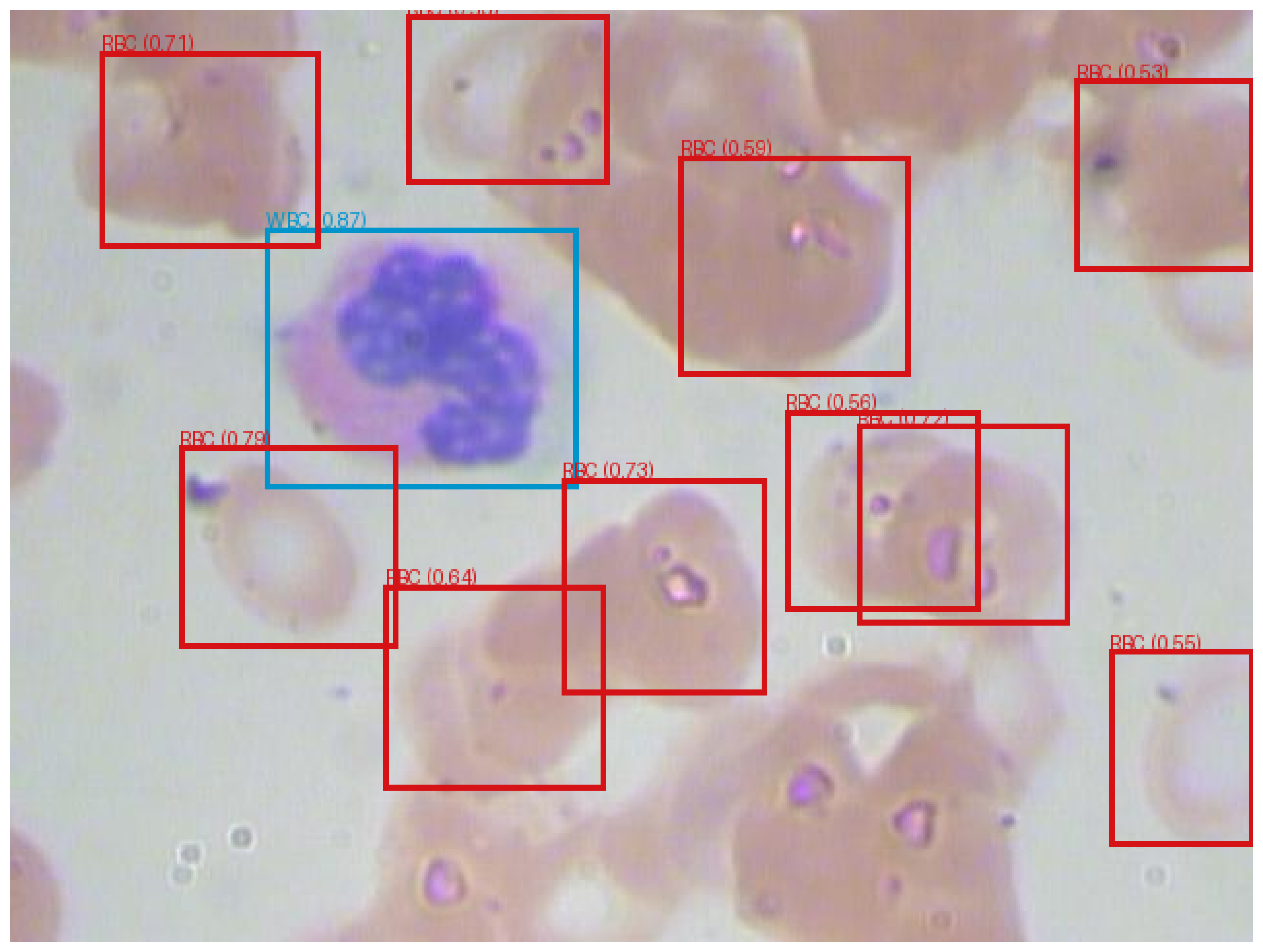
検出されたオブジェクトのバウンディングボックスを入力画像に描画します。その後、PIL および matplotlib ライブラリを使用して、画像とその検出結果を可視化します。
def viz(image_path):
    bboxes, labels, scores = predict(image_path)
    meta_info = [
        {}, # background
        {'class': 'WBC', 'col': '#0094cd'},
        {'class': 'RBC', 'col': '#d51317'},
        {'class': 'Platelets', 'col': '#007b3d'}
    ]

    image = PIL.Image.open(image_path).convert('RGB')
    draw = PIL.ImageDraw.Draw(image)
    for bbox, label, score in zip(bboxes, labels, scores):
        x1, y1, x2, y2 = bbox
        draw.rectangle(((x1, y1), (x2, y2)), outline=meta_info[label]['col'], width=3)
        draw.text((x1, y1 - 10), f'{meta_info[label]["class"]} ({score:.2f})', fill=meta_info[label]['col'])

    fig = plt.figure()
    ax = fig.add_subplot()
    ax.imshow(image)
    ax.axis('off')
    fig.show()
viz('bccd/images/BloodImage_00033.jpg')